The pure C implementation for LeNet5

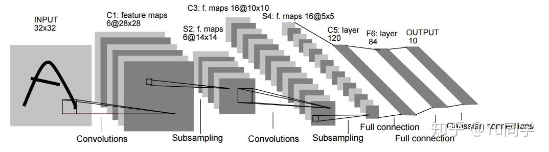
The visualization of LeNet5 structure

[2]

I am recording my LeNet5 C implementation for Intel SGX usage. Because Intel SGX interfaces can only be written in pure C, even C++ would not work. Assume the dataset is MNIST, the size of the black-white image matrix is (1,28,28). The model parameters matrix number group used in the implementation is 3-dimensional. There are 4-dimensional number group in input/output matrices to record the products during the learning process. Note that each channel of the input matrix, owns an independent group of kernel, but each channel’s kernel parameter update share the same total final output of this layer.

How to calculate the matrix size after layer operations:

Convolution

Assumptions:

• The size of input matrix: (dimentional,W,W)
• The size of kernel: (kernel_dimentional, F,F)
• The step size: S
• Padding: P

The size of output matrix size is N.

The meaning of Batch Size

• Batch size is the number of training images between each backward/parameter updates.
• Batch size training can be parallelized with openmp at C. But not work at Intel SGX up to now(I am trying to apply the openmp in Intel SGX at the present).

Convolution implementation

    #define CONVOLUTION_FORWARD(input,output,weight,bias,action)					\
    {																				
      for (int x = 0; x < GETLENGTH(weight); ++x)									\
        for (int y = 0; y < GETLENGTH(*weight); ++y)							\
          CONVOLUTE_VALID(input[x], output[y], weight[x][y]);					\
      FOREACH(j, GETLENGTH(output))												\
        FOREACH(i, GETCOUNT(output[j]))											\
        ((double *)output[j])[i] = action(((double *)output[j])[i] + bias[j]);	\
    }

• The input[x] is the channel of the input matrix.
• The output[y] is the number of feature map for input image’s x channel. For each image’s x channel, the first (for) loop plus each x convolution computation operation to the output[y], and achieve the convolution performance.

Convolution Backward Implementation

  #define CONVOLUTION_BACKWARD(input,inerror,outerror,weight,wd,bd,actiongrad)\
  {																			\
    for (int x = 0; x < GETLENGTH(weight); ++x)								\
      for (int y = 0; y < GETLENGTH(*weight); ++y)						\
        CONVOLUTE_FULL(outerror[y], inerror[x], weight[x][y]);			\
    FOREACH(i, GETCOUNT(inerror))											\
      ((double *)inerror)[i] *= actiongrad(((double *)input)[i]);			\
    FOREACH(j, GETLENGTH(outerror))											\
      FOREACH(i, GETCOUNT(outerror[j]))									\
      bd[j] += ((double *)outerror[j])[i];								\
    for (int x = 0; x < GETLENGTH(weight); ++x)								\
      for (int y = 0; y < GETLENGTH(*weight); ++y)						\
        CONVOLUTE_VALID(input[x], wd[x][y], outerror[y]);				\
  }

• The backward of convolution is indeed the gradient calculation iterated from output layer to input layer, each layer’s gradient depends on the next layer gradient and the layer’s current parameters. From the implementation, we can figure out one shortage of resnet, which originally should make it competitive to Transformer in my opinion. That the res-connection-previous-layer’s gradient in resnet should participate into the res-connection-current-layer’s gradient parameter update on numerial/optimization/mathematical aspect. Due to the limitation of python engineering implementation, such gradient-connection are omitted, and the previous input value simply takes part in the current input. I also would not intend to discuss such missing feature for res-connection at the present thesis work due to the large work-load I have had. But may research it in the future spare time.
• Assume a conv layer in the model, the kernel size is m*m, each output off this layer \(y_{1}.....y_{n}\), would update this layer kernel’s parameters \(\omega_{1}\) …… \(\omega_{m^{2}}\). L is the loss.

For example:

• \(\frac{\partial{y_{j}}}{\partial{\omega_{i}}}\) is the input value that participating into the output value \(y_{j}\)’s calculation, and multiplying by \(\omega_{i}\)

• The kernel parameter update can also follow the convolution-order path, since the sum of the update would not change. For example, the first update:

Backward Parameter update order following convolution order

So backward and forward convolution share the same calculation multiplier:

```C 
    #define CONVOLUTE_VALID(input,output,weight)											
    {																						
      FOREACH(o0,GETLENGTH(output))														
        FOREACH(o1,GETLENGTH(*(output)))												
          FOREACH(w0,GETLENGTH(weight))												
            FOREACH(w1,GETLENGTH(*(weight)))										
              (output)[o0][o1] += (input)[o0 + w0][o1 + w1] * (weight)[w0][w1];
    }
```

Bias Backward Propagation Implementation:

Assume a conv layer in the model, the kernel size is m*m, each output off this layer \(y_{1}.....y_{n}\), would update this layer kernel’s parameters \(\omega_{1}\) …… \(\omega_{m^{2}}\). L is the loss. b denote bias for each output feature map.

Activation backward

• There is a interesting phenomenon for ReLU activation function, that though it is non-linear, if justify is not needed. Because the \(\frac{\partial{ReLU}}{\partial{y}} * \frac{\partial{y}}{\partial{\omega_{i}}} = \frac{\partial{y}}{\partial{\omega_{i}}} = x_{i}\)

• I am wondering during the backward process, if “if-justify” operation is implemented for other types of non-linear activation functions implement, or they use the output directly, or they do not need it just like ReLU.

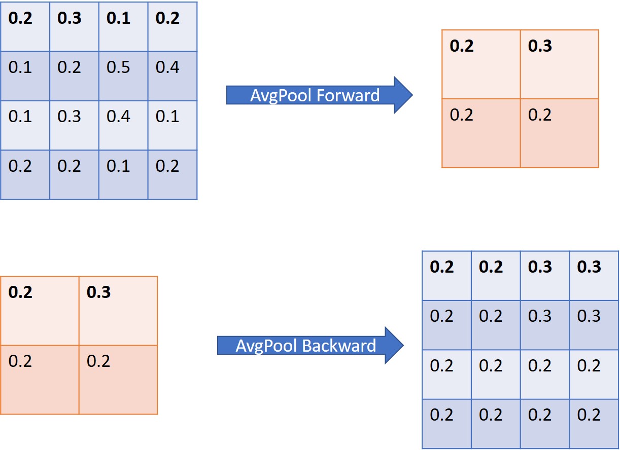
Pooling Backward Propagation Implementation

Max Pooling Backward Mechanism

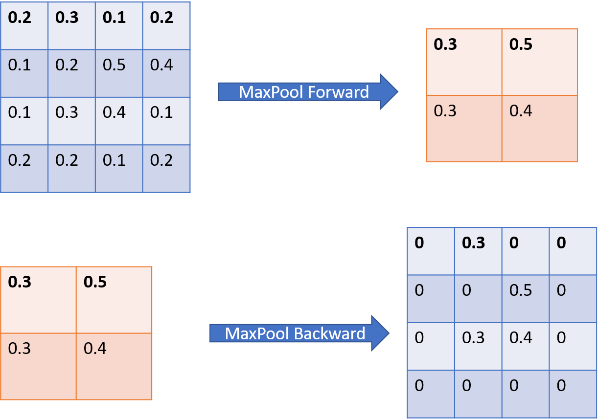
• MaxPooling(Sub-sampling Layer) is used in the LeNet5 implementation

Average Pooling Backward Mechanism

Softmax

  static inline void softmax(double input[OUTPUT], double loss[OUTPUT], int label, int count)
  {
    double inner = 0;
    for (int i = 0; i < count; ++i)
    {
      double res = 0;
      for (int j = 0; j < count; ++j)
      {
        res += exp(input[j] - input[i]);
      }
      loss[i] = 1. / res;
      inner -= loss[i] * loss[i];
    }
    inner += loss[label];
    for (int i = 0; i < count; ++i)
    {
      loss[i] *= (i == label) - loss[i] - inner;
    }
  }

• loss is \(S_{i}\)

Softmax Backward

PreProcessing load_input

• Add padding =2 to input matrix, the output matrix is N = 28+2*2=32. Achieve by create a layer0 matrix with required size of 32,32, then fill in image’s data from 3 to 30(number group from 2 to 29)

• Standardlization and normalization

     static inline void load_input(Feature *features, image input)
     {
       double (*layer0)[LENGTH_FEATURE0][LENGTH_FEATURE0] = features->input;
       const long sz = sizeof(image) / sizeof(**input);
       double mean = 0, std = 0;
       FOREACH(j, sizeof(image) / sizeof(*input))
         FOREACH(k, sizeof(*input) / sizeof(**input))
       {
         mean += input[j][k];
         std += input[j][k] * input[j][k];
       }
       mean /= sz;
       std = sqrt(std / sz - mean*mean);
       FOREACH(j, sizeof(image) / sizeof(*input))
         FOREACH(k, sizeof(*input) / sizeof(**input))
       {
         layer0[0][j + PADDING][k + PADDING] = (input[j][k] - mean) / std;
       }
     }
  

Initial the strcuture of LeNet5

```C
  typedef struct LeNet5
  {
      double weight0_1[INPUT][LAYER1][LENGTH_KERNEL][LENGTH_KERNEL];
      double weight2_3[LAYER2][LAYER3][LENGTH_KERNEL][LENGTH_KERNEL];
      double weight4_5[LAYER4][LAYER5][LENGTH_KERNEL][LENGTH_KERNEL];
      double weight5_6[LAYER5 * LENGTH_FEATURE5 * LENGTH_FEATURE5][OUTPUT];
      /*bias*/
      double bias0_1[LAYER1];
      double bias2_3[LAYER3];
      double bias4_5[LAYER5];
      double bias5_6[OUTPUT];
  }LeNet5;
```

The explanation for C struct LeNet5

C1 Layer

• wegiht0_1: The 1st convolution layer/kernels for the input image(size: 1,32,32), the size of this kernel is: (INPUT=1,LENGTH_KERNEL=5,LENGTH_KERNEL=5), there are LAYER1=6 kernels. The step size is 1. After the first layer, the matrix size would change from (1,28,28) to (Layer1=6, N=28,N=28), consists of 6 feature maps. no padding, padding =0;
• bias0_1: The bias for each kernel at C1 layer, there are LAYER1=6 bias corresponding to each feacture map.
• activation: relu. after each convolution operation. Replace CNN-POOL-RELU with CNN-RELU-POOL process order, the latter one is mostly used in recent cnn applications.

  S2 Layer

  This layer is pure computing operations, and no weights in the layer to compute. So There are no parameters at this layer for LeNet5 C struct. There is no activation function setting for this implementation

  down-sampling layer

  The down-sampling kernel size is (2,2). The output at this layer is 28/kernel_size = (6,14,14), consists of 6 feature maps of size(14,14).

C3 Layer

This is the third layer of LeNet5, a convolutional layer

• weight2_3: LAYER2=6 is the input matrix’s dimentional from S2 Layer. LAYER3=16 is the output matrix’s dimensional from C3 layer. The kernels at this layer is (LAYER3=16, LENGTH_KERNEL = 5,5).
• bias2_3: The bias for the 16 kerners at layer 3.
• Not all feature maps from S2 will be used in C3.

[2] Not all S2's feature maps will be used in C3

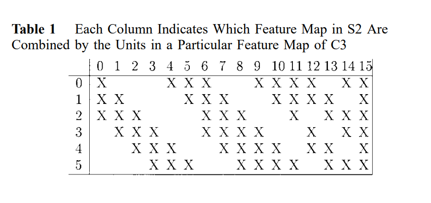
• The implementation does not implement the above connenction throwing.

The data structure of input and output during learning

  typedef struct Feature
  {
    double input[INPUT][LENGTH_FEATURE0][LENGTH_FEATURE0];
    double layer1[LAYER1][LENGTH_FEATURE1][LENGTH_FEATURE1];
    double layer2[LAYER2][LENGTH_FEATURE2][LENGTH_FEATURE2];
    double layer3[LAYER3][LENGTH_FEATURE3][LENGTH_FEATURE3];
    double layer4[LAYER4][LENGTH_FEATURE4][LENGTH_FEATURE4];
    double layer5[LAYER5][LENGTH_FEATURE5][LENGTH_FEATURE5];
    double output[OUTPUT];
  }Feature;

• The INPUT is the channel of input 2-dimensional matrixs. The input is 3-dimensional matrix.

• The Feature data structure is the gradient versus Loss for each parameter in the model.

Reference

• [1] https://zhuanlan.zhihu.com/p/41736894

• [2] https://ieeexplore.ieee.org/stamp/stamp.jsp?tp=&arnumber=726791